In crime analysis, visualising data through maps is essential for understanding patterns and trends. Traditionally, static maps have been commplace across a range of products used to inform police tasking and resource allocation. However, when you’re servicing an entire city or a larger area, creating numerous static maps for inclusion in data products becomes time-consuming.
Enter interactive maps — dynamic tools that allow users to explore data more intuitively with additional details that you’d have to omit from static visuals. This helps us get over limitations, such as:
- inability to scale well when dealing with large datasets or areas
- multiple maps to cover different districts, neighbourhoods or data layers
- end users cannot explore data in-depth
Interactive maps, such as those built with Folium, offer a wide-variety of options for layering multiple insights into a single product, complete with dynamic zoom and pan features, customisable markers, heatmaps, search and draw tools and more (see Folium documentation).
Yet, despite these advantages, setting up interactive maps with Folium can be time-intensive from scratch. Quite often I have spent more time than necessary creating a new map from scratch using snippets of code from prior maps in order to deal with a straight-forward need to show a combination of points and polygons on a map.
Quick Folium
Whilst reading and working through Andrew Wheeler’s book Data Science for Crime Analysis with Python, I was inspired to create a series of functions to save me future time. In Chapter 5, Wheeler demonstrates how to create, store and make effective use of functions, which helped shape my approach in developing modular, reusable tools for mapping crime data in Folium. This text is an invaluable resource for anyone looking to expand their Python skills in the field of crime analysis.
To simplify the process of building interactive crime maps, I’ve developed a series of “Quick Folium” functions (quick_folium.py). These allow analysts to quickly add and style map elements like:
- Map object location: set map location from a geodataframe
- Boundaries: instantly add city, district, neighbourhood or other polygon boundaries
- Points: Easily plot crime incidents or other points of interest; with option to display graduated points such as based on repeat locations
- Heatmaps: visualise crime hotspots
- Labels and popups: provide more context without the need to manually add labels and popups
These can be integrated with existing plugins such as layer control, mini map and draw tools to allow end users to interact.
Walkthrough
The easiest way to use “Quick Folium” functions with Jupyter is to download quick_folium.py from GitHub and store it in the working folder for your project.
# Import what we need
import quick_folium as qf
import folium
from folium import plugins
from folium.plugins import Draw, MiniMap
import geopandas as gpd, requests
from io import BytesIO
We can view the functions and their parameters, so for example, below we can see what the map_location function does.
# View quick folium functions - map_location
help(qf.map_location)

Help on function map_location in module quick_folium:

map_location(gdf)
    Creates centroid for the study area from a geo data frame to use as Folium map location

    Parameters:
    - a geodataframe: a geographic polygon layer.
I have uploaded some sample data to GitHub. Here we will use data from Cleveland Police UK. There are five layers — a districts polygon layer, a neighbourhoods polygon layer, a ward polygon layer, a robbery clusters polygon layer and a robbery points layer for offences falling within the clusters polygon.
# Import data from Github
dist = gpd.read_parquet(BytesIO(requests.get('https://raw.githubusercontent.com/routineactivity/folium_crime_maps/main/sample_data/cp_districts.parquet').content)).to_crs('EPSG:4326')
nbhd = gpd.read_file(BytesIO(requests.get('https://raw.githubusercontent.com/routineactivity/folium_crime_maps/main/sample_data/cp_neighbourhoods.gpkg').content)).to_crs('EPSG:4326')
ward = gpd.read_parquet(BytesIO(requests.get('https://raw.githubusercontent.com/routineactivity/folium_crime_maps/main/sample_data/cp_wards2021.parquet').content)).to_crs('EPSG:4326')
pnts = gpd.read_parquet(BytesIO(requests.get('https://raw.githubusercontent.com/routineactivity/folium_crime_maps/main/sample_data/data_24mrobbery_clusters.parquet').content)).to_crs('EPSG:4326')
clst = gpd.read_parquet(BytesIO(requests.get('https://raw.githubusercontent.com/routineactivity/folium_crime_maps/main/sample_data/data_robbery_clusters.parquet').content)).to_crs('EPSG:4326')
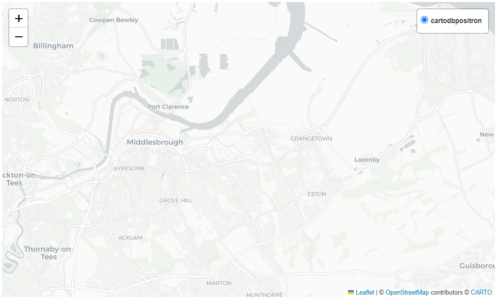
Let’s first create a Folium map object using the map_location function and the layer dist and view the outputs (ironically, each map example that follows is a static screengrab from the interactive output!).
# Use quick folium map_location
m = folium.Map(location=qf.map_location(gdf=dist), zoom_start=12, tiles=None)
folium.TileLayer('CartoDB positron').add_to(m)
folium.LayerControl(collapsed=False).add_to(m)
m
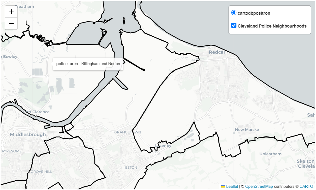
We will now add to this a map_boundary_tooltip using the police neighbourhoods nbhd layer. Our output will be a boundary of the police neighbourhood districts with a popup label.
# Use quick folium map_boundary_tooltip
m = folium.Map(location=qf.map_location(gdf=dist), zoom_start=12, tiles=None)

qf.map_boundary_tooltip(
    map_obj=m,
    geo_data=nbhd,
    fg_name='Cleveland Police Neighbourhoods',
    show=True,
    tooltip_fields=['police_area'],
    popup_fields=['police_area'],
    fo=0,
    fc=None,
    lw=2,
    lc='black',
    name='Cleveland Police Neighbourhoods')

folium.TileLayer('CartoDB positron').add_to(m)
folium.LayerControl(collapsed=False).add_to(m)
m
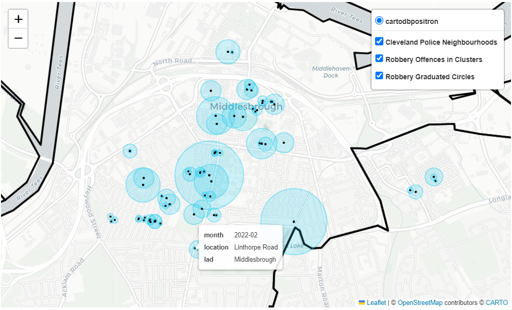
In the next example, we add a point layer of robbery offences using the map_point_label function and pnts layer. We can also create a graduated symbol maps using the pnts layer with the map_graduated_circles function.
# Create multi-layer view - points and graduated points

# Create map using qf.map_location and dist
m = folium.Map(location=qf.map_location(gdf=dist), zoom_start=12, tiles=None)

# Add map_boundary_tooltip with dist geodataframe
qf.map_boundary(
    geo_data=nbhd,
    fg_name='Cleveland Police Neighbourhoods',
    map_obj=m,
    lw=3)

# Add map_point_label with pnts geodataframe
qf.map_point_label(
    map_obj=m,
    geo_data=pnts,
    name='Robbery Offences in Clusters',
    r=6,
    fc='black',
    fo=1,
    ec='black',
    lw=1,
    fields=['month', 'location', 'lad'],
    show=False)

# Add map_graduated_circles with pnts geodataframe
qf.map_graduated_circles(
    map_obj=m,
    gdf_points=pnts,
    radius_scale=15,
    color='#17cbef',
    show=True,
    fill=True,
    fill_color='#17cbef',
    opacity=0.6,
    stroke=True,
    weight=1.0,
    fg_name='Robbery Graduated Circles')

# Add CartoPositron map tile layer and folium layer control
folium.TileLayer('CartoDB positron').add_to(m)
folium.LayerControl(collapsed=False).add_to(m)

# View result
m
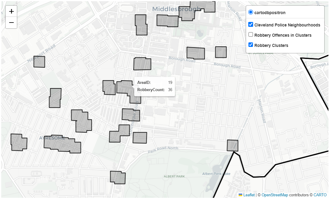
This time, we will map a polygon layer of high robbery clusters and points falling within them. We map the clusters using the map_poly_label function and clst layer. A clusters polygon layer might be the output of an analysis that aims to prioritise micro-locations for police resource deployment, such as hotspot patrols. We may wish to add additional information for end-users about the cluster such as crime data.
# Create multi-layer view - hotspot clusters and points

# Create map using qf.map_location and dist
m = folium.Map(location=qf.map_location(gdf=dist), zoom_start=12, tiles=None)

# Add map_boundary_tooltip with dist geodataframe
qf.map_boundary(
    geo_data=nbhd,
    fg_name='Cleveland Police Neighbourhoods',
    map_obj=m,
    lw=3)

# Add map_point_label with pnts geodataframe
qf.map_point_label(
    map_obj=m,
    geo_data=pnts,
    name='Robbery Offences in Clusters',
    r=6,
    fc='black',
    fo=1,
    ec='black',
    lw=1,
    fields=['month', 'location', 'lad'],
    show=False)

# Add map_poly_label with clst geodataframe
qf.map_poly_label(
    map_obj=m,
    geo_data=clst,
    fg_name='Robbery Clusters',
    lc='black',
    lw=1.5,
    tooltip_fields=['id', 'NUMPOINTS'],
    tooltip_aliases=['AreaID: ', 'RobberyCount: '])

# Add CartoPositron map tile layer and folium layer control
folium.TileLayer('CartoDB positron').add_to(m)
folium.LayerControl(collapsed=False).add_to(m)

# View result
m
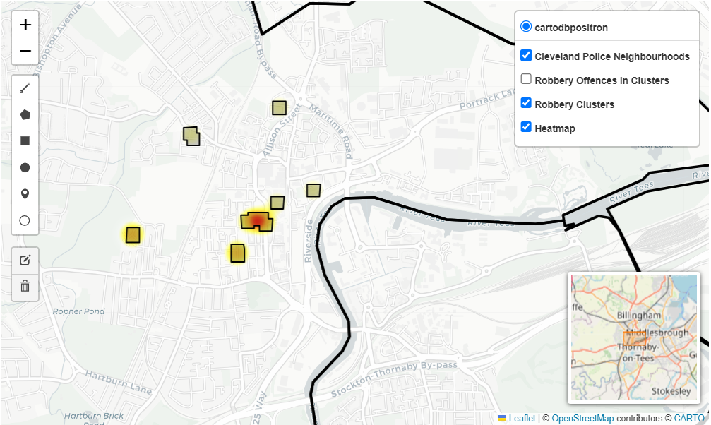
In the final example, we bring together multiple layers in a single output. We add the police neighbourhoods, robbery clusters, points and heatmap. We also add in a MiniMap of the study area and draw tools.
# Final map - hotspot clusters, points and heatmap

# Create map using qf.map_location and dist
m = folium.Map(location=qf.map_location(gdf=dist), zoom_start=12, tiles=None)

# Add map_boundary_tooltip with dist geodataframe
qf.map_boundary(
    geo_data=nbhd,
    fg_name='Cleveland Police Neighbourhoods',
    map_obj=m,
    lw=3)

# Add map_point_label with pnts geodataframe
qf.map_point_label(
    map_obj=m,
    geo_data=pnts,
    name='Robbery Offences in Clusters',
    r=6,
    fc='black',
    fo=1,
    ec='black',
    lw=1,
    fields=['month', 'location', 'lad'],
    show=True)

# Add map_poly_label with clst geodataframe
qf.map_poly_label(
    map_obj=m,
    geo_data=clst,
    fg_name='Robbery Clusters',
    lc='black',
    lw=1.5,
    tooltip_fields=['id', 'NUMPOINTS'],
    tooltip_aliases=['AreaID: ', 'RobberyCount: '])

# Add heatmap_from_points with pnts geodataframe
qf.heatmap_from_points(
    map_obj=m,
    geo_data=pnts,
    fg_name='Heatmap',
    r=15,
    b=10)

# Add CartoPositron map tile layer and folium layer control
folium.TileLayer('CartoDB positron').add_to(m)
folium.LayerControl(collapsed=False).add_to(m)

# Add in a minimap
minimap = plugins.MiniMap()
m.add_child(minimap)

# Add in draw tools
Draw(export=False).add_to(m)

# View result
m
Once complete we can export and save our interactive map as a HTML to share with others.
# Export
m.save("cp-robbery.html")
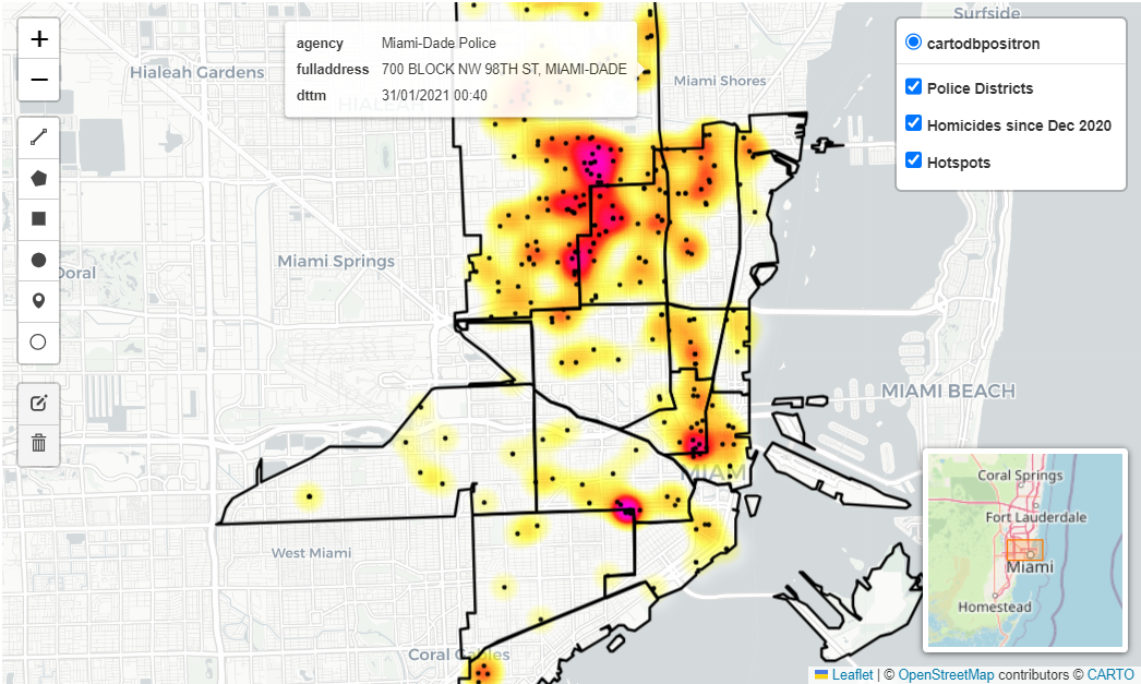
Bonus data and map
Additional data is available for the City of Miami and the Northside area of Miami-Dade.
# Miami data
dist = gpd.read_parquet(BytesIO(requests.get('https://raw.githubusercontent.com/routineactivity/folium_crime_maps/main/sample_data/miami_police_districts2236.parquet').content)).to_crs('EPSG:4326')
homicide = gpd.read_parquet(BytesIO(requests.get('https://raw.githubusercontent.com/routineactivity/folium_crime_maps/main/sample_data/miami_homicide2236.parquet').content)).to_crs('EPSG:4326')
weapons = gpd.read_parquet(BytesIO(requests.get('https://raw.githubusercontent.com/routineactivity/folium_crime_maps/main/sample_data/miami_weapons2236.parquet').content)).to_crs('EPSG:4326')
Links relating to this post
I originally posted this on Medium