Boston Crime Analysis Mini-Project


In this mini-project, I used three tools:
- PostgreSQL with PostGIS for storing geometry (neighbourhoods, police districts, and census tracts) and data tables (crime incidents, shootings).
- Python to crawl, load, and incrementally update the crime and shooting datasets from Analyze Boston.
- Power BI to build a simple interactive dashboard showing trends, hotspots, and patterns.
Step 1: Schema Design in PostgreSQL
Within my local PostgreSQL instance, I spun up a database named usa and defined a boston schema to house all raw and processed tables.
First, I ingested the unaltered CSV exports and shapefiles from Analyze Boston into staging tables alongside the corresponding geometry layers (neighbourhood boundaries, police districts, census tracts). From there, I built a consolidated view that:
- Applies consistent naming and title case
- Normalises timestamp columns to
TIMESTAMP WITH TIME ZONE
- Spatially joins incidents to relevant geographies
- Handles nulls, data types, and adds a custom crime hierarchy
This clean view will be the single source of truth for downstream analysis and visualisation in Power BI. The most recent 12 months will be used for a record-level analysis report page in Power BI.
Additionally, I created a materialised view that aggregates incidents by crime category, police district, and ISO week. By precomputing weekly counts, this view will support a responsive performance report page in Power BI, eliminating the need to query large raw and row-level tables in real time and ensuring fast, seamless rendering of key trends.

Step 2: ETL in Python
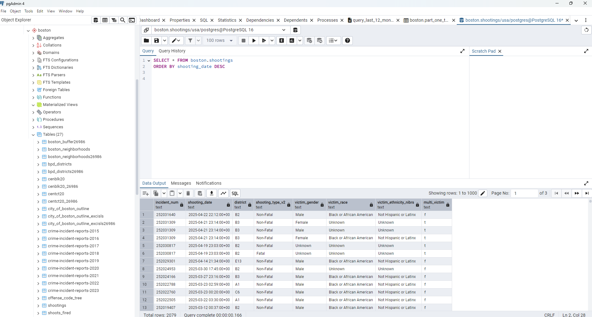
To keep the crime datasets up to date, I needed a way to dynamically retrieve the latest CSV download links from the Analyze Boston data pages, since the URLs change with each dataset refresh. I used Python to scrape the current download links, read the updated data, and append only new rows to the existing PostgreSQL tables for crime incidents and shootings.
To automate the update process, you can schedule the script to run at regular intervals using tools like a Power Automate Desktop flow or a simple .bat file combined with Windows Task Scheduler. The best approach depends on your setup—whether you’re working on a corporate machine with Power Automate access, a personal Windows laptop, or a Linux-based environment where a cron job might be more appropriate.
Scrape URLs.
# Scrape the CSV URLs from Analyze Boston crime incidents
# and shootings pages to keep our tables up to date

import requests
from bs4 import BeautifulSoup
from urllib.parse import urljoin

def fetch_csv_url(page_url):
    r = requests.get(page_url); r.raise_for_status()
    soup = BeautifulSoup(r.text, "html.parser")
    link = soup.find("a", href=lambda h: h and h.endswith(".csv"))
    return urljoin(page_url, link["href"])

crime_url = fetch_csv_url(
    "https://data.boston.gov/dataset/crime-incident-reports-august-2015-to-date-source-new-system"
)
shootings_url = fetch_csv_url(
    "https://data.boston.gov/dataset/shootings/resource/73c7e069-701f-4910-986d-b950f46c91a1"
)

print(crime_url, shootings_url)
Then append new rows.
import pandas as pd
from sqlalchemy import create_engine, text
from io import StringIO

user = "your_username"
password = "your_password"
host = "your_localhost"
port = "your_port_number"
database = "usa"

engine = create_engine(
    "postgresql+psycopg2://{user}:{password}@{host}:{port}/{database}"
)

def update_table(csv_url, table_name):
    res = requests.get(csv_url); res.raise_for_status()
    df = pd.read_csv(StringIO(res.text), low_memory=False)
    # fetch existing keys
    with engine.connect() as conn:
        existing = pd.read_sql(
            text(f"SELECT incident_number FROM boston.{table_name}"),
            conn
        )
    new = df[~df["INCIDENT_NUMBER"].isin(existing["incident_number"])]
    new.columns = new.columns.str.lower()
    if "shooting" in new:
        new["shooting"] = new["shooting"].astype(bool)
    if not new.empty:
        new.to_sql(table_name, engine, schema="boston", if_exists="append", index=False)
        print(f"Inserted {len(new)} new rows into {table_name}")
    else:
        print(f"No new rows for {table_name}")

update_table(crime_url, '"crime_incidents"')
update_table(shootings_url, "shootings")
Step 3: SQL Queries for Power BI
From my PostgreSQL views, I created two key queries to load into Power BI:
One query pulls data from the materialised weekly summary view, optimised for fast rendering of trends and comparisons.
The second query extracts 12 months of record level crime data to support more granular analysis of locations, patterns, and temporal distributions.
In addition, I imported a Boston Police Districts boundary file into Power BI by converting its geometry to WKT format and loading it as a CSV, making it easy to map without requiring direct spatial database connections.
Query for the performance data:
SELECT * FROM boston.part_one_two_weekly_data
Query for the crime trends data:
SELECT
  fid,
  incident_number,
  offense_code,
  offense_code_group,
  offense_description_p,
  custom_group,
  district_nm,
  occurred_timestamp,
  date_from,
  year,
  month,
  day_of_week,
  hour,

  -- 1) round up into 3-hour buckets (0–2→3, 3–5→6 etc)
  CEIL( (hour + 1) / 3.0 ) * 3 AS three_hour_bin,

  -- 2) ISO weekday number (1 = Mon, 2 = Tue etc)
  EXTRACT( ISODOW FROM date_from ) AS weekday_number,

  -- 3) Propercase street + space + district + census tract
  INITCAP(street || ' ' || district_nm || ' ' || ct20) AS street_district,

  street,
  lat,
  long,
  ct20,
  ucr_part,
  shooting_type_v2,
  victim_gender,
  victim_race,
  multi_victim

FROM boston.crime_with_shootings
WHERE date_from >= (
    SELECT MAX(date_from) - INTERVAL '12 months'
    FROM boston.crime_with_shootings
)
  AND date_from <= (
    SELECT MAX(date_from)
    FROM boston.crime_with_shootings
)
Step 4: Building the Power BI Dashboard
This is the fun part! I created two simple report view pages:
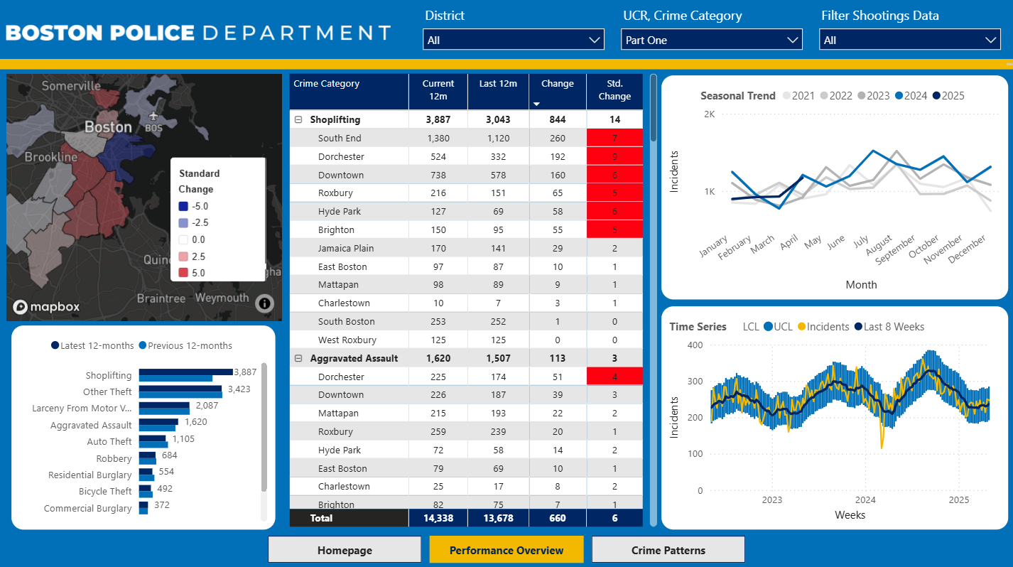
Performance Overview
- Weekly trend line with confidence bands
- Seasonal breakdown (month over year)
- Table summary
- Mapbox choropleth showing % Δ by police district
- Page-wide filters: district, UCR and crime category, shooting flag
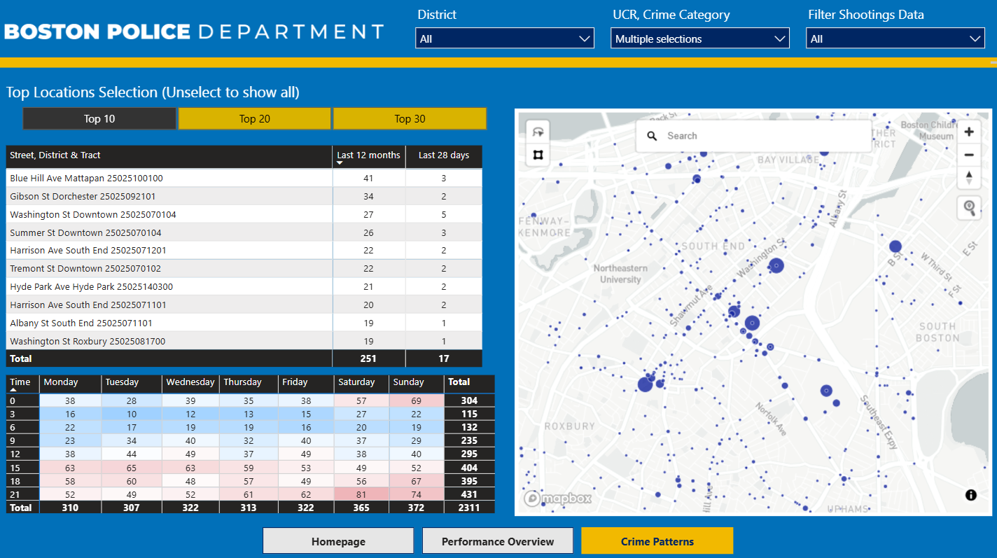
Crime Patterns
- Top 10/20/30 locations by volume
- Table of locations with counts for last 12 months & last 28 days
- Heatmap (hour × weekday)
- Mapbox point map with circle size = count
Report link below, opens in new tab.
👉 View Power BI Report
This mini-project highlights how open data, combined with a few open accessible tools — Python, PostgreSQL, and Power BI — can help deliver timely insights.
I hope this inspires others to explore public datasets and build their own data-driven workflows.
Further reading