The recent Home Office Evaluation report on Grip and bespoke-funded hot spot policing highlighted differences and challenges encountered by analysts in identifying the best hot spot shapes and sizes for their visible policing strategies. Ideally, we want places small enough and hot enough for police officer presence to generate an effect. This short article offers some thoughts when assessing the suitability of the shapes and sizes of hot spots for visible patrol.
This is a follow-up to a previous blog article which considered crime counts versus crime harm
Hot spot shapes
For Op. Grip, police forces had autonomy in determining their spatial units of analysis. A mixture of small grids (boxes or hexagons), Census administrative units (LSOA, Wards), bespoke polygons around hot streets and circular buffers around the central point of an LSOA were used. We can group these into three themes:
- Larger administrative boundaries (LSOA, Ward)
- Uniform micro-places (boxes, hexagons, circles)
- Street segments
Advantages and disadvantages of each
Larger administrative boundaries
- A. Corresponding socio-demographic and economic data aggregated to these same boundaries. This can help match similar places for experimental purposes (i.e. control and treatment comparisons).
- D. Often too large
- D. Most places within them have little or no crime
- D. Policing resources spread thinly which can mean low-intensity intervention dosage.
- D. Statistical bias from high-level aggregation
Uniform micro-places
- A. Uniformity limits statistical bias, the modifiable areal unit problem
- A. Can specify size and shape.
- D. Do not reflect underlying geography and human behaviour patterns.
- D. Cut-off or cut-through streets and hotspots that would naturally be part of a patrol.
- D. May be difficult to generate a large enough number of places with sufficient crime (if the size is too small, or the crime problem is low volume) for a simple randomisation study.
Street segments
- A. Represents a behavioural unit for analysis, consistent with how people use the space.
- A. Large enough to offset imprecise geocoding.
- A. Multiple adjoining hot segments can be clustered together to create larger behavioural units of analysis suitable for statistical blocking.
- A. Can generate time estimates of how long it would take to patrol based on segment lengths.
- D. Cannot obtain socio-demographic and economic data at this level.
- D. It May be difficult to generate a large enough number of segments with a sufficient volume of crime for a simple randomisation study (such as when the crime problem is low volume).
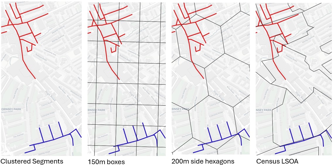
The image below shows how different shapes and sizes of spatial units can appear. Two clusters of high-crime street segments shown in red and blue (which follow the shape and distribution of crimes) are shown on each map. We can see how the hotspot would become dissected when applying grids and administrative boundaries. As the size of the spatial units is increased, there are more low or no crime segments that present within the total potential footprint, which leads us to size and density.
Hot spot size and density
A key challenge noted in the evaluation was that many smaller areas identified for patrols did not have sufficient density of crime to test for statistically significant effects within a single year. When we want to use larger sample sizes, such as for simple random assignment, and our units of analysis are small (i.e. street segments or grids of less than 150m), we can end up selecting lower crime places to achieve enough samples. This can often affect statistical power because of the large variability in place characteristics – very few places have very high counts of serious violent crime (or harm), which was the focus of Grip (homicide, weapon-enabled wounding).
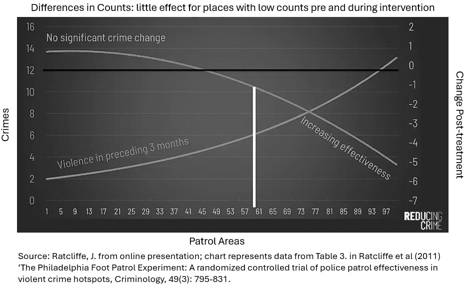
Previous research has found that changes in crime levels during patrol intervention are less effective for places that begin with low pre-intervention counts. The visual above demonstrates this diminishing effect across 120-foot patrol hotspot locations in Philadelphia. Those places above the 60th percentile (61-97 along the x-axis) saw increasing effectiveness of foot patrols. Assessing the pre and during intervention crime counts in this way could help police force areas in England and Wales make decisions about where to draw the cut-off in future hot spot patrol deployments. Looking at the chart, the Philadelphia PD may have chosen the following year to only deploy regular visible patrol at the top 50 rather than 120 locations, for example. This could improve the resources available for higher dosage and intensity in the places where patrol could be most effective.
This isn’t saying ignore the next 50 - you could look at clustering them together to explore opportunities for problem-solving, people-focused or other strategies for example.
Another metric that we can use to help make decisions on size and sufficient density of crime is the Predictive Accuracy Index (PAI). PAI can be calculated for each spatial unit (or ranked groups of units) as the % crime captured (within the study area) divided by the % of geographical area or footprint (of the study area). Different hot spot mapping techniques and spatial units produce different PAI values. We can use these values as a way of guiding our cut-off for areas to be selected for targeting, with a suggested baseline of 10 (Wheeler & Reuter) based on Weisburd’s ‘law of crime concentration (50% of crime typically occurs in 5% of areas).
Using open-source data for the Metropolitan Police UK, I have mapped and calculated PAI values for different spatial units using crimes of Violence and Robbery occurring in 2011-12 (approx. 357,000 offences). The total street-network (in metres) footprint was calculated for each spatial unit and is used as the denominator. The footprint for a patrol using these spatial units ranged from around 88 metres when focused on street segments to around 3,679 metres at the LSOA level.
| Spatial unit |
Total Units |
Max. crime count |
Mean crime count |
Mean network length |
| Segments |
208,866 |
266 |
7 |
88m |
| Squares - 150m boxes |
71,900 |
726 |
5 |
256m |
| Hexagons Uber Res09 - 200m sides |
16,888 |
1,071 |
21 |
1,088m |
| Census LSOA |
4,997 |
2,319 |
71 |
3,679m |
If we think about the optimal patrol times (Koper curve, 15 minutes of patrol) all units in this table other than LSOA are arguably small enough to achieve total coverage in a short patrol.
The places also need to be hot enough and here is where the PAI metric can be used. I have plotted the PAI for the different spatial units to demonstrate how many areas could be suitable for assignment in a visible policing study to address all Violent Crime and Robbery in London.
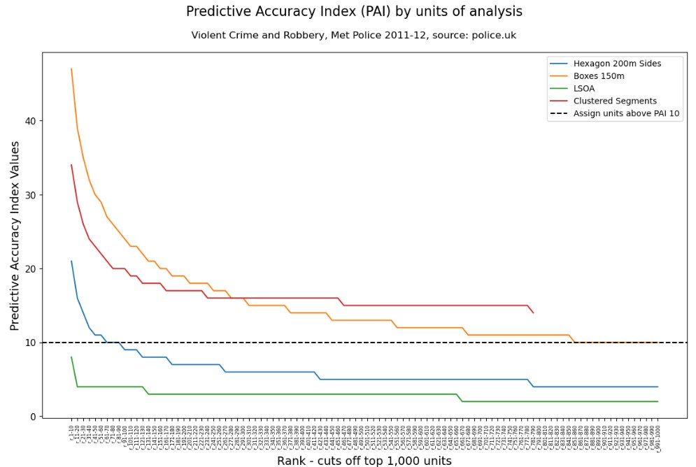
There are two ways we can use the chart as a heuristic to determine cut-offs. The first is taking areas that have a PAI above 10 – in the case of LSOA there were none, and for 200m sided hexagons, there were 90 areas. Smaller units produce many more places beyond a PAI of 10, in which case the ‘elbow curve’ (the point before the PAI values begin to flatline) is where we might consider a cut-off.
In London, for all Violent Crimes and Robbery, the small boxes and clustered segments generated between 160 (clustered segments) and 300 (150m grids) places that would have been eligible for selection for this large volume problem. In reality, we would most likely be using a more refined dataset of street-visible personal crimes much smaller than our broad and limited open data which happens to include many domestic, familial, private settings and even online crimes.
Clustered segments and PAI for the win?
When the intended intervention is visible patrol, shape is perhaps less important than size. Small enough grids (squares, hexagons) can be close to behavioural units of street segments and are the easiest to produce. It might require some additional analysis (overlaying KDE or DBSCAN layers or highlighting the hot segments within the boundaries to focus patrol). My personal preference for visible patrols is clustering high crime street segments together (as appears to have been the method used by Merseyside Police in the Grip evaluation, during which they achieved a 25% reduction in serious violence) because they can produce natural patrol routes for an officer to follow and limit the amount of crime-free or low crime areas that are potentially subject to patrol time.
I cannot say what the optimal size of a hot spot for patrolling should be, although smaller units offer greater precision. Using a PAI assessment can help determine how many places might have a sufficient density of crime. Given that Grip funding was focused on homicide and knife crime, any police forces who were attempting to identify their hotspots using these narrow criteria likely would have found it a challenge to produce many hot spots having a PAI above the suggested baseline and whereby the volumes were stable from one year to the next. The lower volume of serious violence at micro-places shows less stability than higher volumes of all physical violence over time, meaning much attrition of micro hot spots might be expected even without intervention.
Taking into consideration the total footprint of the street network can help think about how long an officer would need to cover a hotspot, and how likely their presence would be noticed - if it requires considerably longer than 15-20 minutes to cover on foot, then is foot patrol the most efficient intervention?
Finally - these thoughts are specific to identifying hot spots for patrol. I do not think that this is the best way to approach the identification of hot spots for other strategies, such as problem-solving at hot spots. Asking analysts to produce problem-solving products for, potentially many, dispersed micro-spaces is likely to result in very ‘shallow’ analyses that can not enable problem-solving.
Further reading
I originally posted this on Medium