This week the Home Office published its Evaluation report on Grip and bespoke-funded hot spot policing, which was the largest national effort in observing and evaluating visible patrol as a strategy to reduce crime in hotspots - in this case high violence locations in England and Wales.
For similarly large-scale national efforts at hotspots, we probably have to go back some way to the Burglary Reduction Initiative (1998-2002, 247 sites, problem-solving at hotspots) and Street Crime Initiative (2002-2004, 10 police forces containing 83% of robbery, problem-solving at hotspots).
In this short article, I’d like to address one of the analytical challenges coming from the evaluation - crime harm versus crime volume for hot spot identification.
Crime harm versus crime volume
Policing has traditionally used crime volumes to identify hot areas. The analysis of crime point data has typically favoured KDE (Kernel Density Estimation), a method that generates aesthetically pleasing smooth surfaces. In recent years, there has been a shift towards experimenting with harm-weighted hotpots, recognising that the impact of offences is not equal across offence types. However, analysts using harm weights have learned that there is a tendency for higher weighted crime, such as a single homicide, to skew selections of the hottest places for intervention.
The Cambridge Crime Harm Index (CCHI) and Crime Severity Score (CSS) both generate weights based on sentencing days (CCHI uses the start point, CSS uses the average), which for a basket of violent crimes can produce weights that range from fewer than 20 for common assault to more than 3,000 for crimes of attempted murder and homicide.
Analytical challenges
When harm-weighted hotspot analyses are conducted using the CCHI/CSS they can produce ‘frequency deserts’ - harm-weighted hotspots where very few or just 1 event has occurred. If our intervention involves patrolling a hotspot, it might not be the best use of resources to send an officer every day to a location where a single isolated event of homicide was the only violent crime to have occurred in a 12-month or longer analytical timeframe.
So why not just use the highest weighted crimes to identify count-based hotspots? Fortunately, events of homicide, attempted murder and weapon-enabled serious wounding occur at relatively low levels in England and Wales. This means that few areas experience space-time clustering of higher weighted crimes within a given year, and those that do are often not stable from one year to the next.
One approach to this problem is to draw on longer-term data and use a recency weighting, but this can still fail to produce small enough areas suitable for hotspot patrol deployments when limited to the lens of homicide, attempted murder and weapon-enabled wounding.
Another is to include similar behavioural problems that are more frequent but lower weighted, such as wounding offences that did not involve the use of knives and firearms. This can produce another type of skew, where concentrated volumes of lower weighted events, such as bar fights in a night-time economy, moderate locations where there is a presence of both higher and lower weighted events.
Further commentary on these challenges is discussed in a recent paper by Vincent Harinam, Zeljko Bavcevic and Barak Ariel: Spatial distribution and development trajectories of crime versus crime severity: do no abandon the count-based model just yet.
(Imperfect) solutions
The solution to removing ‘frequency deserts’, can often be a manual correction. This can be a time burden for someone working in a large urban area or across an entire police force. It can involve making arbitrary cut-off decisions. What do too few offences mean? Less than 10? Less than 1 per week? Less than 1 per month? This can become an iterative loop, which can be fine for a single-time study or intervention, but you do not want to rehash this manual process over and over again.
Something I have experimented with is applying transformations to the raw CCHI/CSS values. The aim is to be able to generate hotspot information that amplifies higher weighted events without generating the frequency deserts. The table below provides an overview of weights that can be applied to a basket of violent crimes, beginning from the raw CCHI value. For example, a homicide is weighted as 5,475 using the CCHI. A log transformation of this value produces a weight of 9 and a square root transformation of this value produces a weight of 74. The count treats all crimes equally.
| Crime type |
CCHI days |
CCHI years |
CCHI Log |
CCHI SQRT |
Count - no weights |
| Homicide |
5,475 |
15.00 |
9 |
74 |
1 |
| Attempted Murder |
3,285 |
9.00 |
8 |
57 |
1 |
| Rape |
1,825 |
5.00 |
8 |
43 |
1 |
| Firearms |
730 |
2.00 |
7 |
27 |
1 |
| Serious Assault |
547 |
1.50 |
6 |
23 |
1 |
| Robbery |
365 |
1.00 |
6 |
19 |
1 |
| Common Assault |
19 |
0.05 |
2 |
3 |
1 |
I have produced visuals to demonstrate the differences in hotspot surfaces produced when applying different transformations of the CCHI. The data is derived from www.crimemapping.com and uses violence, sexual and robbery offences recorded by the Grand Rapids PD in Michigan for the period August 2023 to February 2024. I have added a best-fit CCHI value to each crime category within the dataset.
Comparison maps
All visuals utilise KDE with a consistent spatial bandwidth (550) and cell size (20).
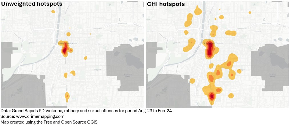
1. Unweighted hotspots (count) vs. CHI weighted (raw values)
The first comparison shows the difference between an unweighted and CHI weighted hotspot surface. This demonstrates why harm weighting has become a consideration as many harmful places are absent using counts alone.
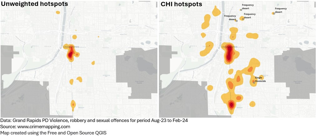
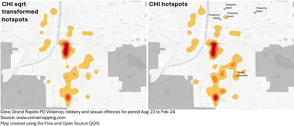
I have added labels in this second map to highlight some of the frequency deserts that the CHI weighted surface has identified.
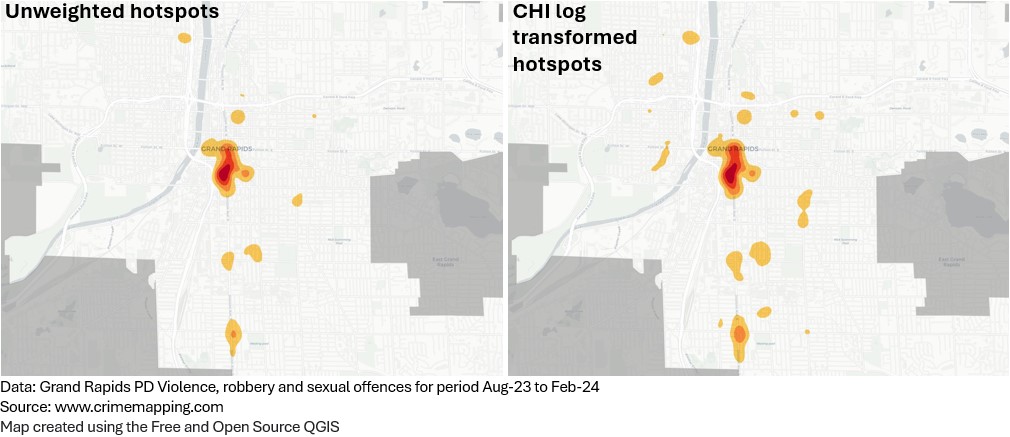
This time the CHI weights have been transformed using a natural logarithm (LN). This more closely resembles the unweighted surface because the new values have been brought much closer together. Here the weighting difference between a homicide (9) and robbery (6) is just three. This amplifies the existing count hotspots, but isn’t emphasising higher weighted events to the extent that we would like it to.
We now transform the CHI weights by taking the square root (SQRT). We can see similarities with the CHI weighted (raw values) surface. Does this solve the problem of frequency deserts?
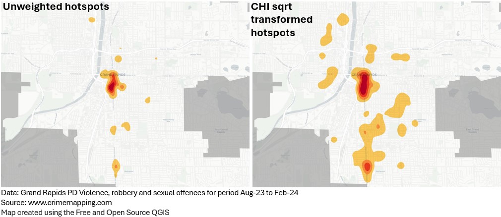
From an exploratory perspective, the square root transform assists in reducing the skew caused by frequency deserts whilst still being able to emphasise harm.
In Grand Rapids, the CCHI square root transform captured 5% more crime counts among the top 10% of its hotspot surface, compared to the top 10% of the surface produced by CCHI values left untransformed. This is the equivalent of up to 300 more crimes.
In terms of harm, there were 732 harm days lost among the top 10% of the CCHI square root transform surface, compared to the top 10% of the CCHI untransformed. This is the equivalent of losing 2x robberies, or 1x firearms incident from the selection of hotspot areas.
More robust testing is no doubt required, but the transformation of harm weights may be a helpful method when applied to spatial point pattern analyses.
Further reading
I originally posted this on Medium