Analysts in policing are frequently asked to prioritise and rank order places and people. Usually, it involves recent data, typically the last 12 months or less, and we expect there will be a disproportionate concentration to focus on. Are these concentrations stable among particular people and places? Are there developmental trends that we can learn from or factor into our selection for targeted intervention?
Group Based Trajectory Modelling (GBTM), aka Group Based Trajectory Analysis (GBTA), is a useful technique for studying trends in offending trajectories or differences in crime patterns in geographic units over time. Below, I present an overview of GBTA, and some walked-through examples applied to crime data using Python.
What is GBTA?
GBTA is the use of longitudinal data to identify distinct trajectory groups.
In criminal justice, this usually means a person’s developmental pattern (criminal career) over age and time. However, it can also be applied to geography. I first came across GBTA in ‘Criminology of Place’ which observed trends in crime for each of Seattle’s street segments over 16 years.
What might we use it for?
When applied to person data, we can use GBTA to understand when patterns of offending increase, decline and become inactive. We can conduct further analyses of distinct group trajectories. This might be to understand how patterns vary by age, types of offending behaviour and differences between types of offenders.
In geographical places, our aim could be understanding which few places drive increases and reductions in crime, or those places which present perennial challenges that require longer-term place strategies to change.
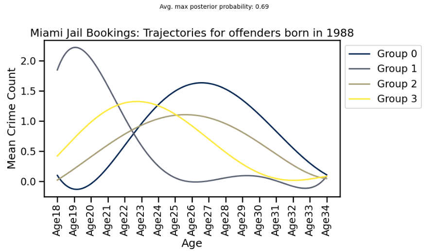
The example below uses open data from Miami Jail Bookings on person offending leading to arrest. Here we can see four distinct trajectories in offending across all people in the dataset born in 1988. For illustrative purposes, we might label Group 1 as “desisters” — they offended frequently in their late teens, but then tailed off rapidly thereafter remaining low.
Doing GBTA. What’s involved?
The basic steps in a GBTA are:
- Summarise data into rows containing unique persons/places and columns containing crime counts by time (i.e. age for persons, or calendar years for places)
- Choose a model type based on the data distribution (Zero Inflated Poisson, Gaussian or cnorm)
- Determine the number of groups (order of the model)
- Determine the nature of groups (places, crime types, cohorts)
The GBTA will attempt to group individuals or places with similar patterns over time.
For a more detailed explanation, I recommend watching David Nagin’s ‘Workshop in Methods: Group-Based Trajectory Models An Overview’ lecture.
GBTA: London UK Robbery 2011-2023
With data from police.uk I aggregated London robberies 2011–2023 into 450m square grids then generated a GBTA using these as my spatial units of analysis. Nine distinct trajectories were generated. You can see these in the visual below (a small group of cells in the West End of London are excluded as this group had significantly higher mean counts).
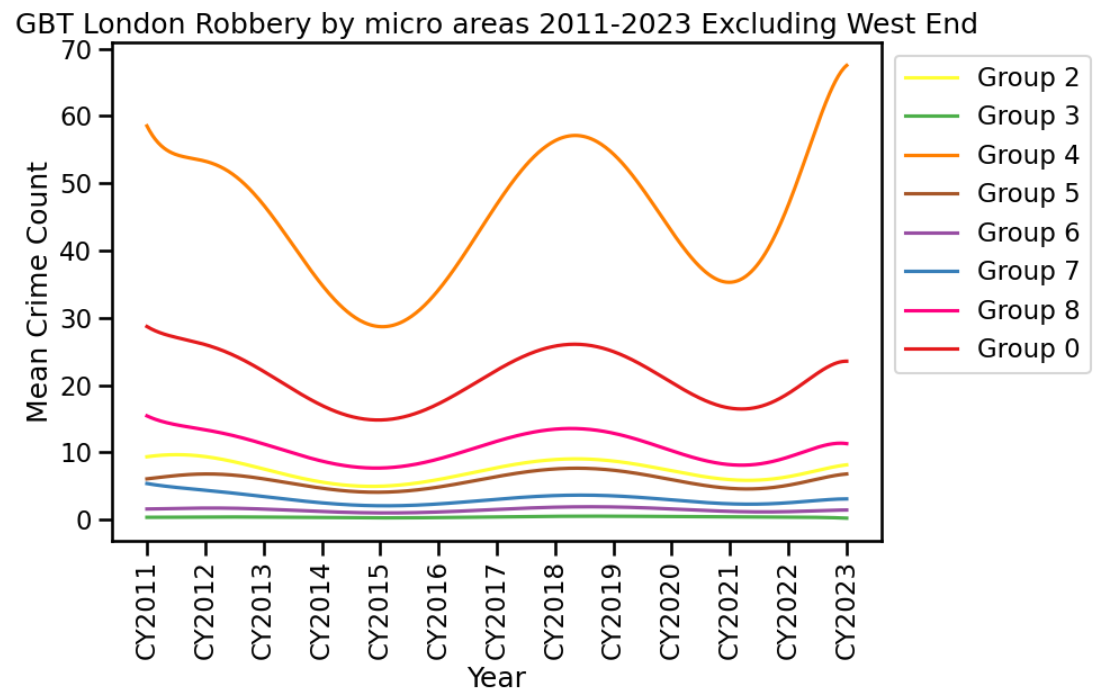
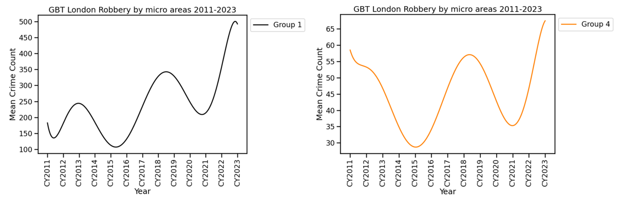
Each trajectory in the chart shows the average number of crimes for 450m square grids belonging to a group. For example, spatial units in Group 4 as of 2023 had a mean robbery count of almost 70 and this is the highest mean for the group since 2011. The areas in Group 4 saw a falling trend post the 2011 riots, with subsequent increases and falls during Covid occurring in 2020–21.
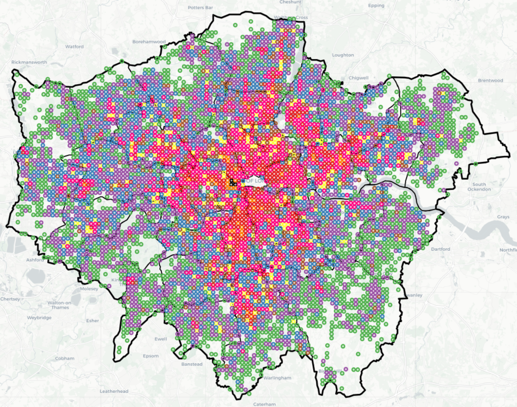
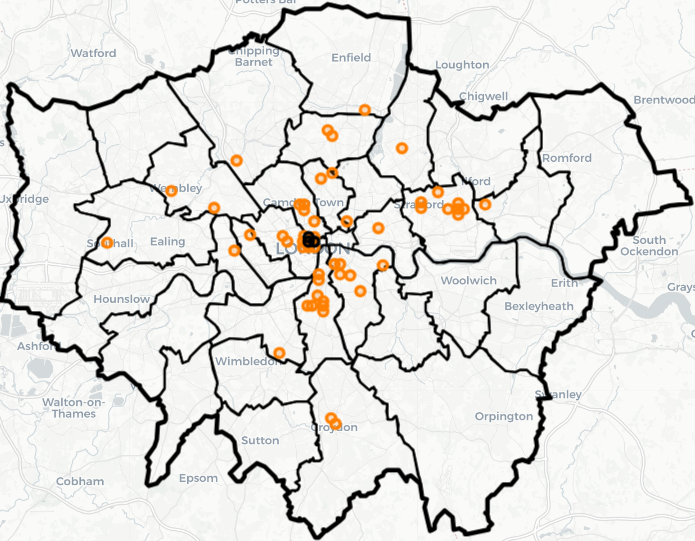
These groups can be viewed geographically in the map below. An interactive version of this map can be viewed here.
At one end of the scale are Group 1 and Group 4.
Group 1 which is just three 450m grid squares within London’s West End had the highest means for robbery, with a steep increase here post-Covid. There were almost 10,000 robberies since 2011 contributing to nearly 3% of all robberies in the dataset.
Group 4, with 52 450m grid squares, saw a mean robbery count of nearly 70 in 2023. There were over 32,000 robberies in these locations since 2011 accounting for 8% of the total.
Group 1 and 4 locations are shown below.
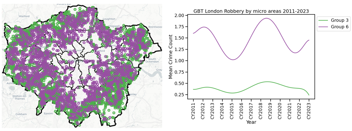
At the opposite end of the scale are Group 3 and Group 6. Locations in Group 3 frequently have less than 1 robbery offence per year, and Group 6 has less than 2 robberies per year. These groups make up 53% of London’s geographical area and contain 10% of robberies since 2011.
Whilst Group 1 and Group 4 are perhaps obvious candidates for targeted robbery reduction efforts, even making significant improvements in those areas is unlikely to drastically move the dial in robbery volumes at the city-wide level.
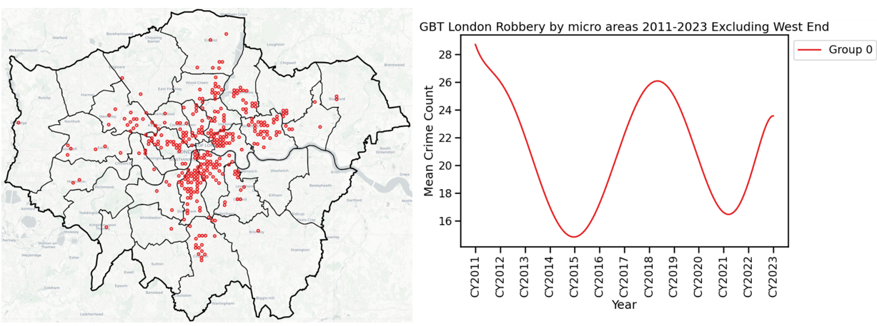
Finally, Group 0, whereby we might describe robbery levels as moderately high, contributed notably to the peaks and troughs in overall robbery volumes across London. At their highest, the micro-spaces (450m square grids) in this group had around 1 crime per fortnight. This group is 5% of London’s geographical area and 25% of all robberies (93,000 since 2011).
Geographically Group 0 areas often clump together to create possible contiguous places from which to form larger target areas (combined with Groups 1 and 4) for problem-solving and place-based strategies.
GBTA does not have to limit itself to uniform polygons. For example, it could be applied to street segment data (as done in the Weisburd et al study of Seattle) to produce more precise target area boundaries that capture the extent of crime patterns.
Below I provide the basic code used in this example to generate GBTA. You can also find materials used from GitHub at this link. More advanced GBTA examples and other software (R, Stata) examples are provided at the end of this article.
Code Block 1: modules used and data import/reshape
# what's needed
import pandas as pd
import numpy as np
from hmmlearn import hmm
from sklearn.model_selection import train_test_split
from sklearn.metrics import silhouette_score
import matplotlib.pyplot as plt
import seaborn as sns
#read in data from here https://github.com/routineactivity/gbtm_examples/tree/main/london_robbery
df = pd.read_csv('grid450m_robbery_counts.csv')
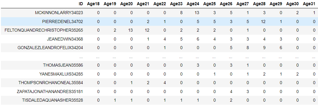
df.head()
#reshape data
data_for_hmm = df.iloc[:, 1:].values
lengths = [len(row) for row in data_for_hmm]
data_for_hmm = np.concatenate(data_for_hmm).reshape(-1, 1)
Code Block 2: running the GBTA
# fit HMM return BIC for given number of groups
def fit_hmm(n_groups):
    model = hmm.PoissonHMM(n_groups=n_groups, n_iter=100, random_state=42)
    model.fit(data_for_hmm, lengths=lengths)
    return model, model.bic(data_for_hmm)

# determine best n groups based on BIC
best_model, best_bic, best_n_groups = None, float('inf'), 0
for n_groups in range(7,10):
    model, bic = fit_hmm(n_groups)
    if bic < best_bic:
        best_bic = bic
        best_model = model
        best_n_groups = n_groups

# assign each geographic place /or individual if using person data/ to a group
group_assignments = np.split(best_model.predict(data_for_hmm), np.cumsum(lengths)[:-1])

# extract probabilities for each place/individual for each group
group_probabilities = np.split(best_model.predict_proba(data_for_hmm), np.cumsum(lengths)[:-1])
Code Block 3: reshaping and merging results to original data for plotting and mapping
# results with IDs for interpretable table view
results = pd.DataFrame({
    'ID': df['ID'],
    'Group': [assignment[0] for assignment in group_assignments],
    'Probabilities': [prob[0] for prob in group_probabilities]
})

# output results
best_n_groups, results.head()

# generate results dataframe for export
ids = df['ID'].values
group_assignments_flat = [assignment[0] for assignment in group_assignments]
max_probs = [np.max(prob[0]) for prob in group_probabilities]

# results as df
results_df = pd.DataFrame({
    'ID': ids,
    'Group': group_assignments_flat,
    'MaxPosteriorProbability': max_probs
})

# merge with original data
df_with_results = pd.merge(df, results_df, on='ID')
df_with_results
Further reading
I originally posted this on Medium