The Home Office Clear, Hold, Build (CHB) initiative is a place-focused intervention that has been happening in England and Wales since 2021. In a recent impact evaluation, analysts used a four-stage approach — combining Propensity Score Matching (PSM), Synthetic Control Method (SCM), Parallel Trends Assessment, and Difference-in-Differences (DID) — to assess whether the intervention effectively reduced crime.
Note:This article is not a full review of the CHB initiative, nor is it intended as a primer on PSM, SCM, and DID. For an accessible introduction to causal inference methods, please see Scott Cunningham’s https://mixtape.scunning.com/
1. Overview of the Home Office CHB Impact Evaluation
Before launching the impact evaluation, an exercise was undertaken to identify which socio-economic factors best explain the geographical distribution of total crime in England and Wales. An Ordinary Least Squares (OLS) model revealed that the following seven variables are strong predictors of total crime:
- White residents
- Living with deprivation indicators
- Usual residents
- Economically active
- In managerial occupations
- With no qualifications
- Country of birth UK
Note: It is unclear which spatial units (possibly Lower Super Output Areas, or LSOAs) were used and whether spatial dependencies (e.g., spatial lag or error models) were considered.
Stage 1:
After identifying key socio-economic predictors, PSM was used to match CHB pilot sites with comparable non-CHB areas within the same police force jurisdiction. Importantly, crime outcome measures were not included in the matching process.
To illustrate this step, I obtained open data for the Merseyside Police Force area. Three CHB sites in Merseyside were approximated as follows:
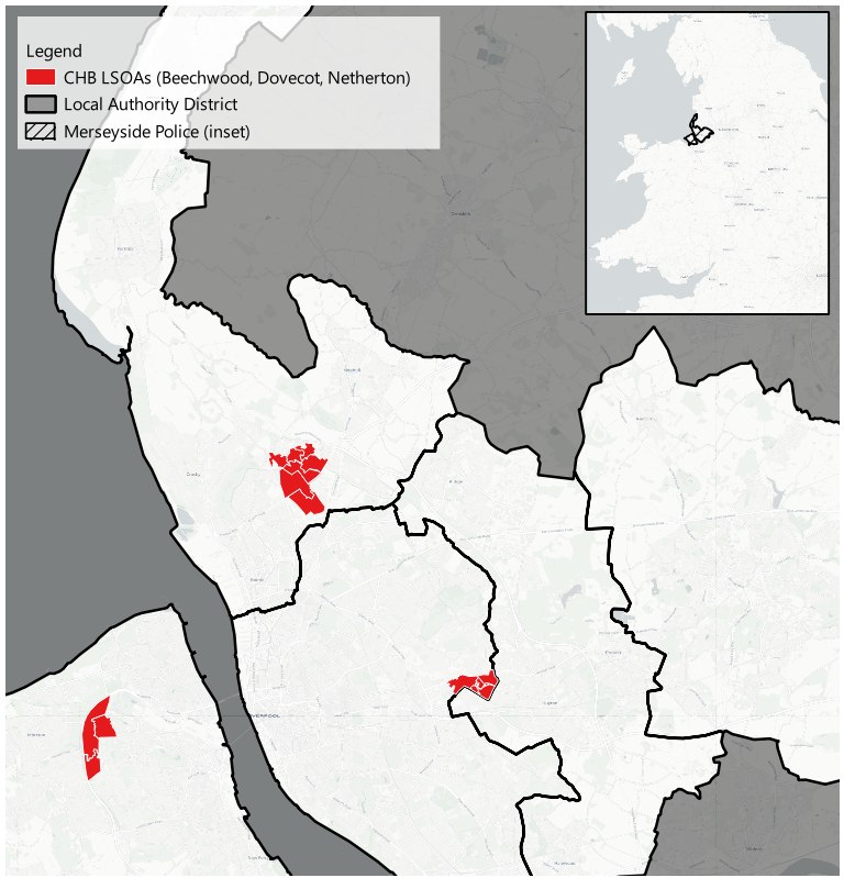
Since the exact boundaries were unavailable, a set of LSOAs was used to approximate these CHB areas. A dataset of socio-economic variables for every LSOA in the Merseyside area was then compiled and used to generate PSM matches for the CHB sites.
Access the dataset here.
The following Python code demonstrates a basic implementation of PSM using the psmpy package:
import pandas as pd
url = 'https://github.com/routineactivity/adhoc_notebooks/blob/main/chb_psm_scm/data/df_psm.csv?raw=true'
df_psm = pd.read_csv(url)
# copy columns we need
df = df_psm[['index', 'treatment', 'residents', 'ec_active', 'non_white', 'manager',
'no_qualifications', 'unemployed']].copy()
# import relevant libraries
from psmpy import PsmPy
from psmpy.functions import cohenD
from psmpy.plotting import *
# set the dataframe, treatment column and index column - should be integer, and initialize the class
psm = PsmPy(df, treatment='treatment', indx='index', exclude = [])
# calculate logit/ps scores
psm.logistic_ps(balance = False)
# view the raw values
psm.predicted_data
# matching with knn one to many
psm.knn_matched_12n(matcher='propensity_logit', how_many=5)
# distribution of lsoas by logit score, treatment and control
psm.plot_match(Title='Side by side matched controls', Ylabel='Number of LSOAs', Xlabel= 'Propensity logit', names = ['treatment', 'control'], colors=['#C8102E', '#003399'] ,save=True)
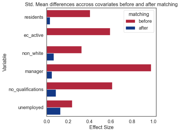
# plot effect size differences
psm.effect_size_plot(title='Std. Mean differences accross covariates before and after matching', before_color='#C8102E', after_color='#003399', save=False)
The resulting balance of covariates before and after PSM (comparable to Table 3 in the Home Office Impact Evaluation Technical Annex) confirms that the matching process has improved the similarity between treatment (CHB) and control LSOAs.
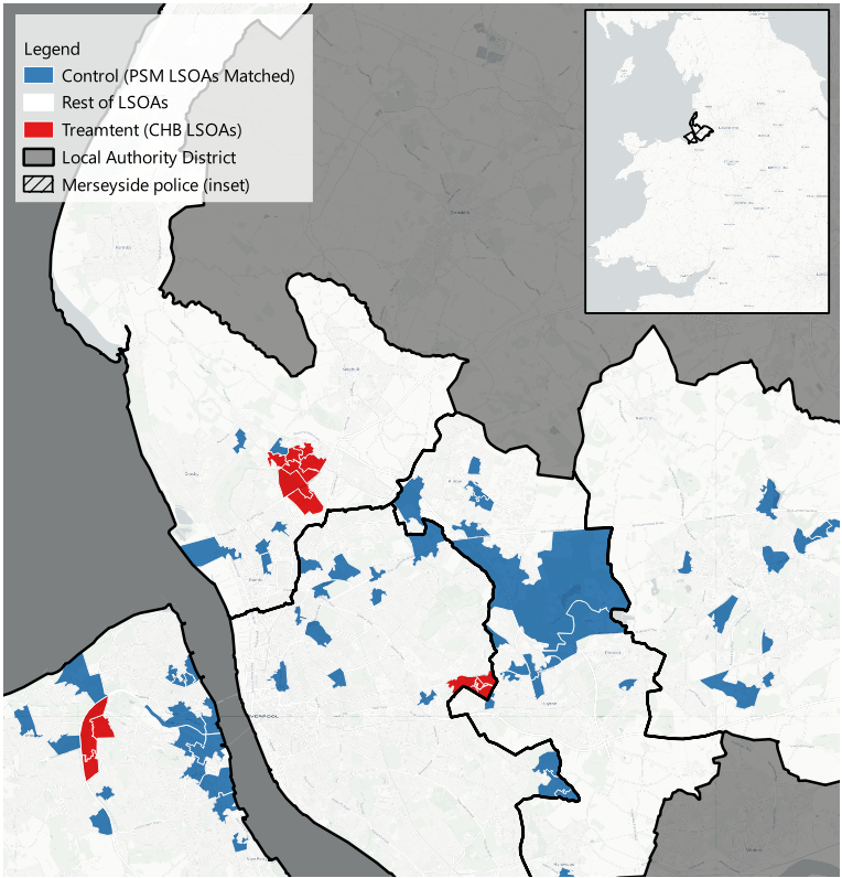
These matched IDs are then re-integrated into the original dataset to form a refined set of treatment (CHB) and control (non-CHB) LSOAs.
The map below illustrates the identified LSOAs — CHB sites are in red and the PSM-matched control LSOAs are in blue.
If needed, applying an exclusion zone (e.g., to prevent spillover effects) requires a corresponding data column to denote adjacent neighbours for exclusion during matching.
Stage 2:
The PSM process was based solely on socio-economic variables and did not account for crime rates. Experience shows that good socio-demographic matching does not always translate to well-matched crime trends. In some studies, PSM is enhanced by including the crime outcome as a matching variable for targeted and problem-focused initiatives (see Braga et al. 2019; Chainey et al. 2022). However, for broader analyses assessing multiple crime outcomes, PSM alone may be insufficient.
To better align the crime trends between CHB sites and control areas, SCM was employed to construct a synthetic control — a weighted combination of control units that best mimics the pre-intervention crime trajectory of the treated unit.
A crime dataset for both CHB and control LSOAs in Merseyside was created using data from police.uk. This dataset includes:
- LSOA ID
- Month (as a period variable)
- Crime type counts
- Binary indicator for the intervention period (1= intervention, 0 = pre-intervention)
- Binary indicator for treatment status (1=CHB Site, 0=control)
For this walkthrough, the intervention period is defined as starting on January 1, 2023.
Access the dataset here.
The following Python code outlines the SCM process, which is repeated for each crime type. In this example, a Lasso regression is used to optimally weight the donor pool.
import pandas as pd
import numpy as np
from sklearn.impute import SimpleImputer
from sklearn.linear_model import Lasso
import os
url = 'https://github.com/routineactivity/adhoc_notebooks/blob/main/chb_psm_scm/data/crime_data_psm_matches_v2.csv?raw=true'
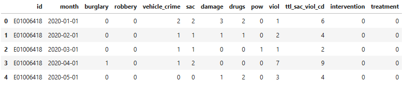
df = pd.read_csv(url)
# Convert the 'month' column to datetime format
df['month'] = pd.to_datetime(df['month'])
df.head()
# define count cols to loop through
count_columns = df.columns[2:11]
# create a dictionary to save plots and dataframes
output_dir = r'C:/Users/Username/Folder/chb_merseyside/psm_matched_scm'
if not os.path.exists(output_dir):
os.makedirs(output_dir)
for col in count_columns:
# filter data for current column
temp_data = df[['id', 'month', col, 'treatment', 'intervention']].copy()
# filter control data and pivot
inverted = (temp_data.query("treatment == 0 and intervention == 0")
.pivot(index='id', columns='month')[[col]]
.T)
# prepare y (treat) and x (control)
y = temp_data.query("treatment == 1 and intervention == 0").groupby('month')[col].sum().values
X = inverted.values
# handle NaNvalues in X
imputer = SimpleImputer(strategy='mean')
X = imputer.fit_transform(X)
# fit lasso regression
lasso = Lasso(alpha=0.1, fit_intercept=False, max_iter=100000)
lasso.fit(X, y)
weights_lr = lasso.coef_
# generate synth using weights
synth_lr = (temp_data.query("treatment == 0")
.pivot(index='month', columns='id')[col]
.values.dot(weights_lr))
# prepare results df
treated_data_sum = temp_data.query("treatment == 1").groupby('month')[col].sum().reset_index()
result = pd.DataFrame({
'month': treated_data_sum['month'],
'actual_treated': treated_data_sum[col],
'synthetic_control': synth_lr
}).set_index('month')
# save data
result.to_csv(f'{output_dir}/{col}_data.csv')
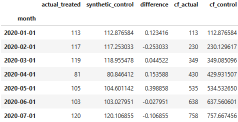
For each crime type, this process produces a results data frame that includes:
- actual_treated: CHB site crime counts
- synthetic_control: Weighted crime counts from the donor pool (the counterfactual)
- Cumulative frequency values (cf_actual and cf_control): These can also be computed to provide additional insight.
Stage 3:
Two methods were used to evaluate the synthetic control:
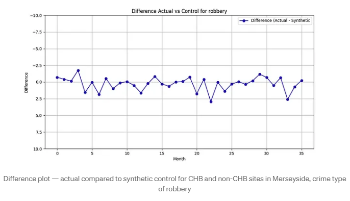
- Visual Inspection of Pre-Intervention Trends
A plot of the difference between the actual CHB crime counts and the synthetic control helps assess stability.
# calculate difference
result['difference'] = result['actual_treated'] - result['synthetic_control']

# result pre
result_pre = result.query("month < '2023-01-01'").reset_index()

# plot difference between actual and synthetic
plt.figure(figsize=(12,6))
plt.plot(result_pre.index, result_pre['difference'], label='Difference (Actual - Synthetic', color='#1a0dab', marker='o')
#plt.axvline(x=intervention_start, color='#000000', linestyle=':', label='Intervention Start')
plt.xlabel('Month')
plt.ylabel('Difference')
plt.ylim(10,-10)
plt.title(f'Difference Actual vs Control for {col}')
plt.legend()
plt.grid(True)
plt.savefig(f'{output_dir}/{col}_diff_plot.png')
plt.close()
For example, a difference plot for robbery reveals that the pre-intervention discrepancies are consistently small (roughly between –2.5 and 2.5), indicating a good match.
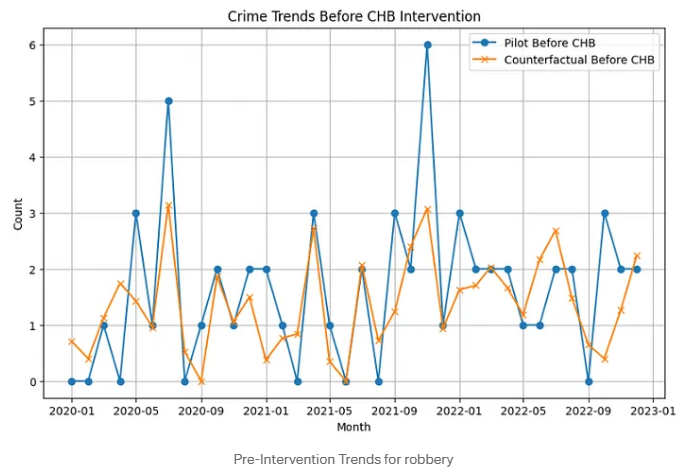
We can also visualise the raw values month to month.
Note: the impact evaluation generated rolling crime rates to visually inspect the quality of the match, unlike the coarser monthly values displayed below.
- Event Study Analysis
An event study regression (using a linear model) is employed to formally test for pre-intervention differences. In this regression, the absence of a significant trend in the difference between actual and synthetic data supports the validity of the synthetic control.
Note: The Technical Annex of the Home Office Impact Evaluation goes into significant detail on this process.
import statsmodels.api as sm

# If not already in the df, add a difference column and time variable
df['time'] = (df['month'] - df['month'].min()).dt.days
df['difference'] = df['actual_treated'] - df['synthetic_control']

# fit linear regression difference ~ time
X = sm.add_constant(df['time'])
model = sm.OLS(df['difference'], X).fit()
print(model.summary())
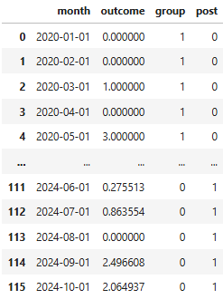
Stage 4:
The final stage employs a standard DiD specification. First, the results data frame is reshaped to a long format and binary indicators are added for group (1 = CHB site, 0 = control) and period (1 = post-intervention, 0 = pre-intervention).
The following code snippet shows the basic DiD approach using statsmodels:
import statsmodels.formula.api as smf

model = smf.ols("outcome ~ group + post + group:post", data=df_long).fit()
print(model.summary())
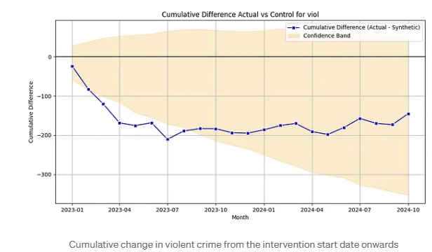
In the model summary, the coefficient of the interaction term (group:post) provides the DiD estimate—that is, the change in crime at CHB sites post-intervention relative to the control group. Visual representations, such as cumulative frequency plots (inspired by Andrew Wheeler’s Crime De-Coder), can further aid in interpreting these results. For example, a plot of violent crime data from Merseyside shows a significant reduction in the first eight months post-intervention.
2. Using PSM and SCM together?
Should PSM Restrict the Donor Pool?
A key question is whether PSM should be used to pre-select the donor pool before constructing the synthetic control. My prior experience suggests that socio-economic and demographic variables may not fully capture the dynamics underlying crime outcomes. By performing PSM first, there is a risk of discarding areas that might otherwise provide a better pre-treatment fit when used in SCM.
In Merseyside, where there are 923 LSOAs, the CHB evaluation used 14 CHB LSOAs and 70 PSM-matched controls. In contrast, SCM (as outlined by Abadie et al. 2010 and Cunningham 2021) can draw on a much richer donor pool — even including areas that differ in socio-demographics — to create a synthetic match that closely replicates the outcome trajectory of treated units.
3. SCM with and without PSM
I conducted two sets of SCM analyses:
- PSM-Matched Donor Pool: Where controls were selected using PSM.
- Full Donor Pool: Where all untreated LSOAs (approximately 900+ in Merseyside) were included.
Parallel Trends
When using the PSM-matched donor pool, some crime types (e.g., possession of weapons and robbery) exhibited larger deviations in pre-intervention trends, suggesting less alignment.
In contrast, the full donor pool produced near-zero interaction coefficients and nearly perfect pre-trend correlations, indicating a superior match.
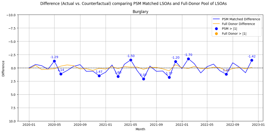
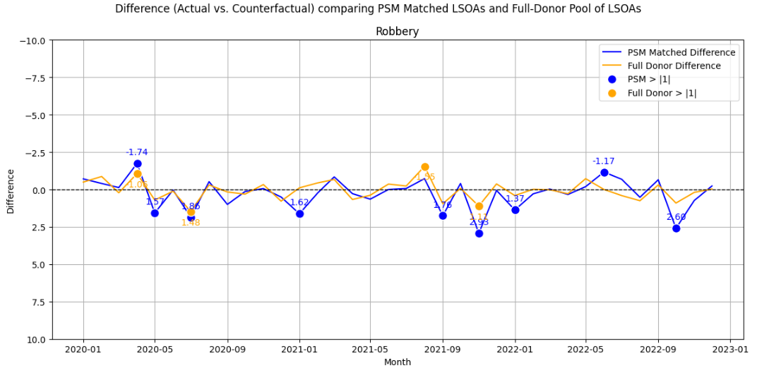
A visual inspection of the parallel trends for burglary and robbery, which had lower correlations, is shown below. In the first plot, Burglary, we can see multiple deviations +/- 1 in the PSM-matched donor, but none for the full donor. A second plot for Robbery is shown. This is a lower volume event, with both methods experiencing deviations, less so for the full donor.
Difference-in-Difference Estimates
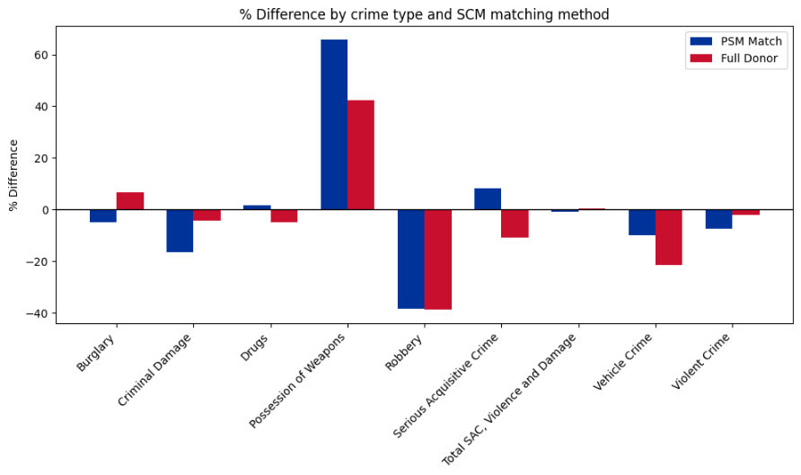
While most p-values were high (suggesting non-significant differences between CHB and control sites), some crime types (such as robbery) showed similar estimated effects between the two methods.
Other crime types (e.g., possession of weapons, vehicle crime, burglary, drugs, and serious acquisitive crime) displayed notable differences in effect magnitude — or even direction — depending on whether PSM was applied beforehand.
These results raise an important question: if the full donor pool produces better parallel trends, can we consider its DiD estimates more credible?
How donor pools are defined will undoubtedly influence the analysis. Therefore, analysts must carefully assess which approach yields the most valid counterfactual.
Conclusion
This walkthrough has provided a simplified overview of how the Home Office CHB impact evaluation might be executed “under the hood.” By integrating PSM with SCM, and then assessing synthetic control quality through visual and formal methods before finally applying DiD analysis, we can better understand the potential benefits — and pitfalls — of different donor pool strategies.
While using a full donor pool appears to offer superior pre-intervention matching, the choice between a PSM-restricted pool and an unrestricted pool has implications for the credibility of the final estimates. Future research should continue to examine these trade-offs to guide best practices in place-based crime intervention evaluations.
See also
Reading on Clear, Hold, Build
ChatGPT was used to help improve the clarity, structure and flow of this written article.
I originally posted this on Medium